Productivity Gains

As already mentioned, base cost and transfer cost both represent the unit manufacturing cost of a product. The base cost is the unit cost that was specified when the project was developed by R&D, for a first production batch of 100,000 units. The transfer cost of a product is the real unit cost to bear (i.e. price paid by the Marketing center to the Production center) and is initially equal to the base cost of its R&D project, as long as the production batch is 100,000 units.

The transfer cost usually digresses from the base cost. The reason is that manufacturing costs tend to decrease over time thanks to the experience effect. Transfer cost (per unit) will decrease over time because of experience effects: as the production center produces more and more units (high cumulative volume of production), benefits of experience are observed: labor efficiency leads to fewer mistakes in the production process, processes and methodologies are improved, new and less expensive materials are used, … As a consequence, the (unit) transfer cost decreases as the cumulative volume of production increases.

Hence, one way to reduce manufacturing costs is simply to produce more units of the same product. On average, you can expect the transfer cost to be reduced by 15% each time the cumulative production of a given product gets doubled. This is represented by the blue curve on Figure 7:

• Suppose that a base cost of $150 was specified by the R&D (at the development of the project) for a production of 100,000 units (point A);

• A few periods later, if cumulative production has doubled compared to the initial batch of 100,000 units (i.e. 200,000 units have been produced so far), the (unit) transfer cost will be around $127 (15% less than the initial $150) (point C).

• Each time cumulative production doubles, the (unit) transfer costs decreases by 15%: at cumulative production = 400,000 units, the transfer cost would be around 108 (15% less than $127 at 200,000 units); at cumulative production = 800,000 units, the transfer cost would be around 92 (15% less than $108 at 400,000 units). In other words, the additional production necessary to get an additional 15% reduction in unit cost gets bigger and bigger (as it is no linear relationship). On Figure 6, point B represents the transfer cost when cumulative production reached 600,000 units. When compared to the initial base cost, the unit cost of this brand only decreased from $150 to $100 (a 33% reduction), showing that the slope of the experience curve decreases quite rapidly.

  Experience effect also involves that if your cumulative production is less than the production batch of 100,000 units, the product transfer cost will be higher than the initial base cost specified when the project was developed by R&D. As a rule of thumb, you can expect the transfer cost to be higher by about 15% if the cumulative production of a given product is 50,000 units, i.e. half the initial production batch of 100,000 units.

  Finally, be aware of the fact that costs will be adjusted for inflation; but companies won’t actually observe any cost increase, as this impact will be offset by the reduction obtained through experience, as cumulative production increases at each period (unless production is 0; in that case, the average transfer cost will increase by the inflation rate, ususally around 2%).

  Experience effect should not be confused with economies of scale, where manufacturing costs decrease with the size of the production, as fixed costs are amortized on large production batches, negotiation power with suppliers is higher, investment in machines of varying sizes and speeds ensures higher usage ratio, access to less expensive financing is made possible, … As the Marketing department is not responsible for production capacity, you are not concerned with economies of scale.

  Firms can further reduce manufacturing costs by launching a cost reduction R&D project, i.e. a project specifying the same physical characteristics as the initial project, but at a lower base cost. This is represented by the red curve on Figure 7. Although the unit cost will initially be higher than $100 (point A’), the curve shows that transfer costs below $100 will be obtained as soon as cumulative production goes beyond point B’. Then, the transfer costs will be much lower than the ones achievable by the original blue curve.

  

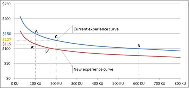
  Figure 7 – Productivity gains